How to Read Decision Tree Plot Python

one.10. Decision Copse¶

Decision Trees (DTs) are a non-parametric supervised learning method used for classification and regression. The goal is to create a model that predicts the value of a target variable by learning uncomplicated decision rules inferred from the data features. A tree tin be seen as a piecewise constant approximation.

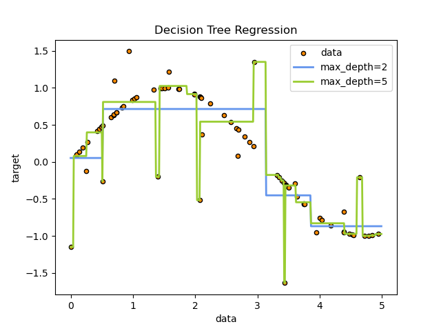
For case, in the example beneath, decision trees acquire from data to guess a sine curve with a ready of if-then-else determination rules. The deeper the tree, the more complex the determination rules and the fitter the model.

Some advantages of decision trees are:

• Uncomplicated to understand and to interpret. Trees tin can exist visualised.

• Requires fiddling data preparation. Other techniques often require information normalisation, dummy variables need to be created and blank values to exist removed. Note still that this module does non support missing values.

• The cost of using the tree (i.e., predicting data) is logarithmic in the number of data points used to railroad train the tree.

• Able to handle both numerical and categorical data. However scikit-learn implementation does non support chiselled variables for now. Other techniques are commonly specialised in analysing datasets that have simply ane type of variable. Run into algorithms for more information.

• Able to handle multi-output problems.

• Uses a white box model. If a given state of affairs is observable in a model, the explanation for the condition is hands explained past boolean logic. Past contrast, in a blackness box model (e.thousand., in an artificial neural network), results may be more difficult to interpret.

• Possible to validate a model using statistical tests. That makes information technology possible to business relationship for the reliability of the model.

• Performs well even if its assumptions are somewhat violated by the true model from which the data were generated.

The disadvantages of conclusion copse include:

• Determination-tree learners can create over-complex trees that practice non generalise the data well. This is called overfitting. Mechanisms such as pruning, setting the minimum number of samples required at a leaf node or setting the maximum depth of the tree are necessary to avoid this problem.

• Decision trees can be unstable considering small variations in the data might result in a completely dissimilar tree being generated. This problem is mitigated by using decision copse within an ensemble.

• Predictions of decision trees are neither smoothen nor continuous, but piecewise constant approximations as seen in the above figure. Therefore, they are not good at extrapolation.

• The trouble of learning an optimal conclusion tree is known to be NP-complete under several aspects of optimality and even for elementary concepts. Consequently, applied conclusion-tree learning algorithms are based on heuristic algorithms such as the greedy algorithm where locally optimal decisions are made at each node. Such algorithms cannot guarantee to return the globally optimal decision tree. This can be mitigated by grooming multiple trees in an ensemble learner, where the features and samples are randomly sampled with replacement.

• There are concepts that are hard to learn because decision trees do not express them easily, such as XOR, parity or multiplexer problems.

• Determination tree learners create biased copse if some classes dominate. It is therefore recommended to balance the dataset prior to plumbing equipment with the conclusion tree.

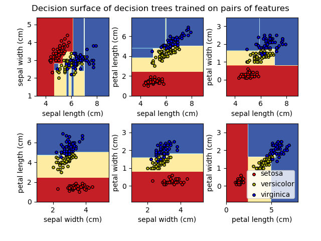
ane.10.one. Classification¶

DecisionTreeClassifier is a class capable of performing multi-class classification on a dataset.

Every bit with other classifiers, DecisionTreeClassifier takes as input two arrays: an array 10, sparse or dense, of shape (n_samples, n_features) holding the training samples, and an array Y of integer values, shape (n_samples,) , belongings the class labels for the training samples:

                            >>>                            from              sklearn              import              tree              >>>                            X              =              [[              0              ,              0              ],              [              1              ,              1              ]]              >>>                            Y              =              [              0              ,              ane              ]              >>>                            clf              =              tree              .              DecisionTreeClassifier              ()              >>>                            clf              =              clf              .              fit              (              X              ,              Y              )            

Subsequently being fitted, the model can then exist used to predict the course of samples:

                            >>>                            clf              .              predict              ([[              2.              ,              ii.              ]])              array([1])            

In example that there are multiple classes with the same and highest probability, the classifier will predict the grade with the lowest alphabetize among those classes.

As an alternative to outputting a specific class, the probability of each class can be predicted, which is the fraction of training samples of the grade in a leaf:

                            >>>                            clf              .              predict_proba              ([[              ii.              ,              2.              ]])              assortment([[0., 1.]])            

DecisionTreeClassifier is capable of both binary (where the labels are [-1, one]) classification and multiclass (where the labels are [0, …, One thousand-ane]) classification.

Using the Iris dataset, we can construct a tree as follows:

                            >>>                            from              sklearn.datasets              import              load_iris              >>>                            from              sklearn              import              tree              >>>                            iris              =              load_iris              ()              >>>                            Ten              ,              y              =              iris              .              data              ,              iris              .              target              >>>                            clf              =              tree              .              DecisionTreeClassifier              ()              >>>                            clf              =              clf              .              fit              (              X              ,              y              )            

Once trained, you tin plot the tree with the plot_tree function:

                            >>>                            tree              .              plot_tree              (              clf              )              [...]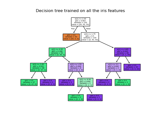            

We can also export the tree in Graphviz format using the export_graphviz exporter. If you lot use the conda package managing director, the graphviz binaries and the python package can be installed with conda install python-graphviz .

Alternatively binaries for graphviz can be downloaded from the graphviz projection homepage, and the Python wrapper installed from pypi with pip install graphviz .

Below is an case graphviz consign of the in a higher place tree trained on the unabridged iris dataset; the results are saved in an output file iris.pdf :

                            >>>                            import              graphviz              >>>                            dot_data              =              tree              .              export_graphviz              (              clf              ,              out_file              =              None              )              >>>                            graph              =              graphviz              .              Source              (              dot_data              )              >>>                            graph              .              render              (              "iris"              )            

The export_graphviz exporter also supports a variety of aesthetic options, including coloring nodes past their grade (or value for regression) and using explicit variable and class names if desired. Jupyter notebooks also render these plots inline automatically:

                            >>>                            dot_data              =              tree              .              export_graphviz              (              clf              ,              out_file              =              None              ,              ...                            feature_names              =              iris              .              feature_names              ,              ...                            class_names              =              iris              .              target_names              ,              ...                            filled              =              True              ,              rounded              =              Truthful              ,              ...                            special_characters              =              Truthful              )              >>>                            graph              =              graphviz              .              Source              (              dot_data              )              >>>                            graph            

Alternatively, the tree can too be exported in textual format with the office export_text . This method doesn't require the installation of external libraries and is more compact:

                            >>>                            from              sklearn.datasets              import              load_iris              >>>                            from              sklearn.tree              import              DecisionTreeClassifier              >>>                            from              sklearn.tree              import              export_text              >>>                            iris              =              load_iris              ()              >>>                            decision_tree              =              DecisionTreeClassifier              (              random_state              =              0              ,              max_depth              =              2              )              >>>                            decision_tree              =              decision_tree              .              fit              (              iris              .              data              ,              iris              .              target              )              >>>                            r              =              export_text              (              decision_tree              ,              feature_names              =              iris              [              'feature_names'              ])              >>>                            print              (              r              )              |--- petal width (cm) <= 0.80              |   |--- class: 0              |--- petal width (cm) >  0.fourscore              |   |--- petal width (cm) <= one.75              |   |   |--- form: 1              |   |--- petal width (cm) >  1.75              |   |   |--- form: 2            

1.x.ii. Regression¶

Decision trees can also be practical to regression problems, using the DecisionTreeRegressor class.

As in the nomenclature setting, the fit method will take as argument arrays Ten and y, only that in this case y is expected to accept floating point values instead of integer values:

                            >>>                            from              sklearn              import              tree              >>>                            X              =              [[              0              ,              0              ],              [              2              ,              two              ]]              >>>                            y              =              [              0.5              ,              two.5              ]              >>>                            clf              =              tree              .              DecisionTreeRegressor              ()              >>>                            clf              =              clf              .              fit              (              Ten              ,              y              )              >>>                            clf              .              predict              ([[              ane              ,              one              ]])              assortment([0.5])            

1.10.3. Multi-output issues¶

A multi-output problem is a supervised learning problem with several outputs to predict, that is when Y is a 2d assortment of shape (n_samples, n_outputs) .

When at that place is no correlation between the outputs, a very simple way to solve this kind of problem is to build n independent models, i.due east. one for each output, and so to utilize those models to independently predict each 1 of the n outputs. Yet, because information technology is likely that the output values related to the same input are themselves correlated, an oftentimes amend way is to build a single model capable of predicting simultaneously all n outputs. First, information technology requires lower training time since only a single figurer is built. Second, the generalization accuracy of the resulting estimator may often exist increased.

With regard to decision trees, this strategy can readily be used to support multi-output problems. This requires the following changes:

• Store due north output values in leaves, instead of one;

• Use splitting criteria that compute the boilerplate reduction across all north outputs.

This module offers support for multi-output bug by implementing this strategy in both DecisionTreeClassifier and DecisionTreeRegressor . If a conclusion tree is fit on an output array Y of shape (n_samples, n_outputs) then the resulting calculator will:

• Output n_output values upon predict ;

• Output a list of n_output arrays of class probabilities upon predict_proba .

The employ of multi-output trees for regression is demonstrated in Multi-output Conclusion Tree Regression. In this example, the input X is a single real value and the outputs Y are the sine and cosine of 10.

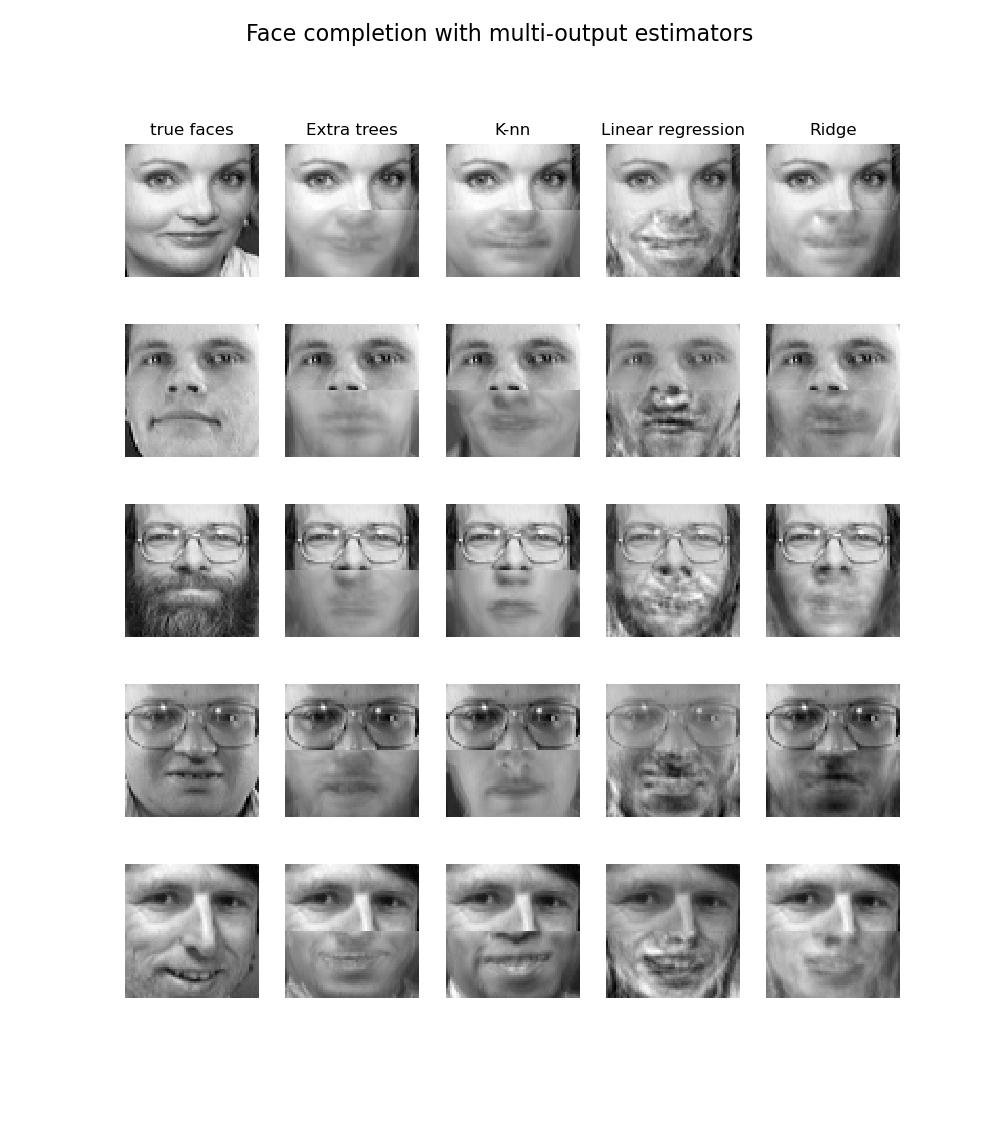
The apply of multi-output trees for classification is demonstrated in Face completion with a multi-output estimators. In this example, the inputs X are the pixels of the upper half of faces and the outputs Y are the pixels of the lower half of those faces.

i.10.4. Complexity¶

In full general, the run time price to construct a balanced binary tree is \(O(n_{samples}n_{features}\log(n_{samples}))\) and query fourth dimension \(O(\log(n_{samples}))\). Although the tree structure algorithm attempts to generate counterbalanced trees, they will non always exist balanced. Assuming that the subtrees remain approximately balanced, the cost at each node consists of searching through \(O(n_{features})\) to discover the characteristic that offers the largest reduction in entropy. This has a cost of \(O(n_{features}n_{samples}\log(n_{samples}))\) at each node, leading to a total toll over the unabridged copse (past summing the cost at each node) of \(O(n_{features}n_{samples}^{2}\log(n_{samples}))\).

1.10.5. Tips on practical utilize¶

• Decision trees tend to overfit on data with a big number of features. Getting the right ratio of samples to number of features is important, since a tree with few samples in high dimensional space is very likely to overfit.

• Consider performing dimensionality reduction (PCA, ICA, or Feature pick) beforehand to give your tree a amend chance of finding features that are discriminative.

• Understanding the determination tree structure will aid in gaining more insights well-nigh how the decision tree makes predictions, which is important for understanding the important features in the data.

• Visualise your tree equally you are training by using the export function. Use max_depth=3 equally an initial tree depth to become a experience for how the tree is fitting to your data, and so increase the depth.

• Recollect that the number of samples required to populate the tree doubles for each additional level the tree grows to. Use max_depth to control the size of the tree to preclude overfitting.

• Apply min_samples_split or min_samples_leaf to ensure that multiple samples inform every decision in the tree, by decision-making which splits will be considered. A very small number will normally mean the tree volition overfit, whereas a large number will preclude the tree from learning the data. Try min_samples_leaf=5 as an initial value. If the sample size varies greatly, a float number can be used as percentage in these two parameters. While min_samples_split can create arbitrarily small leaves, min_samples_leaf guarantees that each foliage has a minimum size, avoiding low-variance, over-fit foliage nodes in regression problems. For nomenclature with few classes, min_samples_leaf=1 is often the best choice.

  Note that min_samples_split considers samples directly and independent of sample_weight , if provided (e.g. a node with m weighted samples is withal treated equally having exactly m samples). Consider min_weight_fraction_leaf or min_impurity_decrease if accounting for sample weights is required at splits.

• Residual your dataset earlier training to prevent the tree from being biased toward the classes that are dominant. Class balancing can be done by sampling an equal number of samples from each class, or preferably by normalizing the sum of the sample weights ( sample_weight ) for each class to the same value. Also note that weight-based pre-pruning criteria, such as min_weight_fraction_leaf , will and so be less biased toward dominant classes than criteria that are non aware of the sample weights, like min_samples_leaf .

• If the samples are weighted, information technology will be easier to optimize the tree construction using weight-based pre-pruning criterion such as min_weight_fraction_leaf , which ensure that leaf nodes comprise at to the lowest degree a fraction of the overall sum of the sample weights.

• All determination trees use np.float32 arrays internally. If grooming data is not in this format, a copy of the dataset will be fabricated.

• If the input matrix X is very thin, it is recommended to convert to sparse csc_matrix before calling fit and sparse csr_matrix before calling predict. Training fourth dimension can be orders of magnitude faster for a sparse matrix input compared to a dense matrix when features accept zippo values in most of the samples.

1.10.6. Tree algorithms: ID3, C4.5, C5.0 and CART¶

What are all the diverse decision tree algorithms and how do they differ from each other? Which one is implemented in scikit-learn?

ID3 (Iterative Dichotomiser 3) was developed in 1986 by Ross Quinlan. The algorithm creates a multiway tree, finding for each node (i.eastward. in a greedy manner) the chiselled characteristic that volition yield the largest information gain for chiselled targets. Trees are grown to their maximum size and then a pruning step is usually applied to improve the ability of the tree to generalise to unseen data.

C4.5 is the successor to ID3 and removed the brake that features must exist categorical by dynamically defining a detached attribute (based on numerical variables) that partitions the continuous attribute value into a discrete set up of intervals. C4.5 converts the trained trees (i.e. the output of the ID3 algorithm) into sets of if-and so rules. These accuracy of each rule is and so evaluated to make up one's mind the order in which they should exist practical. Pruning is done by removing a rule's precondition if the accuracy of the dominion improves without it.

C5.0 is Quinlan'due south latest version release under a proprietary license. It uses less memory and builds smaller rulesets than C4.5 while being more than accurate.

CART (Nomenclature and Regression Trees) is very similar to C4.five, simply it differs in that it supports numerical target variables (regression) and does non compute dominion sets. CART constructs binary trees using the feature and threshold that yield the largest information proceeds at each node.

scikit-learn uses an optimised version of the CART algorithm; still, scikit-learn implementation does not support categorical variables for now.

1.x.7. Mathematical formulation¶

Given training vectors \(x_i \in R^n\), i=1,…, fifty and a label vector \(y \in R^l\), a decision tree recursively partitions the feature space such that the samples with the same labels or similar target values are grouped together.

Let the data at node \(thousand\) be represented by \(Q_m\) with \(N_m\) samples. For each candidate split \(\theta = (j, t_m)\) consisting of a characteristic \(j\) and threshold \(t_m\), division the data into \(Q_m^{left}(\theta)\) and \(Q_m^{correct}(\theta)\) subsets

\[ \begin{marshal}\begin{aligned}Q_m^{left}(\theta) = \{(x, y) | x_j <= t_m\}\\Q_m^{right}(\theta) = Q_m \setminus Q_m^{left}(\theta)\cease{aligned}\end{align} \]

The quality of a candidate split up of node \(m\) is then computed using an impurity function or loss function \(H()\), the choice of which depends on the task being solved (classification or regression)

\[G(Q_m, \theta) = \frac{N_m^{left}}{N_m} H(Q_m^{left}(\theta)) + \frac{N_m^{right}}{N_m} H(Q_m^{correct}(\theta))\]

Select the parameters that minimises the impurity

\[\theta^* = \operatorname{argmin}_\theta 1000(Q_m, \theta)\]

Recurse for subsets \(Q_m^{left}(\theta^*)\) and \(Q_m^{right}(\theta^*)\) until the maximum allowable depth is reached, \(N_m < \min_{samples}\) or \(N_m = one\).

one.10.7.1. Classification criteria¶

If a target is a classification outcome taking on values 0,1,…,K-i, for node \(yard\), let

\[p_{mk} = ane/ N_m \sum_{y \in Q_m} I(y = g)\]

exist the proportion of class k observations in node \(m\). If \(m\) is a final node, predict_proba for this region is set to \(p_{mk}\). Mutual measures of impurity are the post-obit.

Gini:

\[H(Q_m) = \sum_k p_{mk} (1 - p_{mk})\]

Entropy:

\[H(Q_m) = - \sum_k p_{mk} \log(p_{mk})\]

Misclassification:

\[H(Q_m) = i - \max(p_{mk})\]

1.10.vii.2. Regression criteria¶

If the target is a continuous value, so for node \(grand\), mutual criteria to minimize as for determining locations for future splits are Mean Squared Error (MSE or L2 mistake), Poisson deviance also as Mean Absolute Error (MAE or L1 error). MSE and Poisson deviance both set the predicted value of terminal nodes to the learned mean value \(\bar{y}_m\) of the node whereas the MAE sets the predicted value of concluding nodes to the median \(median(y)_m\).

Mean Squared Error:

\[ \brainstorm{align}\brainstorm{aligned}\bar{y}_m = \frac{1}{N_m} \sum_{y \in Q_m} y\\H(Q_m) = \frac{i}{N_m} \sum_{y \in Q_m} (y - \bar{y}_m)^ii\end{aligned}\end{align} \]

Half Poisson deviance:

\[H(Q_m) = \frac{i}{N_m} \sum_{y \in Q_m} (y \log\frac{y}{\bar{y}_m} - y + \bar{y}_m)\]

Setting criterion="poisson" might be a good option if your target is a count or a frequency (count per some unit). In any instance, \(y >= 0\) is a necessary condition to use this criterion. Note that it fits much slower than the MSE criterion.

Mean Absolute Error:

\[ \brainstorm{align}\begin{aligned}median(y)_m = \underset{y \in Q_m}{\mathrm{median}}(y)\\H(Q_m) = \frac{1}{N_m} \sum_{y \in Q_m} |y - median(y)_m|\terminate{aligned}\end{align} \]

Annotation that it fits much slower than the MSE criterion.

1.ten.8. Minimal Cost-Complexity Pruning¶

Minimal cost-complexity pruning is an algorithm used to clip a tree to avoid over-fitting, described in Chapter three of [BRE]. This algorithm is parameterized by \(\alpha\ge0\) known as the complication parameter. The complexity parameter is used to define the cost-complication measure out, \(R_\alpha(T)\) of a given tree \(T\):

\[R_\alpha(T) = R(T) + \blastoff|\widetilde{T}|\]

where \(|\widetilde{T}|\) is the number of concluding nodes in \(T\) and \(R(T)\) is traditionally defined as the full misclassification rate of the terminal nodes. Alternatively, scikit-larn uses the full sample weighted impurity of the terminal nodes for \(R(T)\). Equally shown to a higher place, the impurity of a node depends on the benchmark. Minimal cost-complexity pruning finds the subtree of \(T\) that minimizes \(R_\alpha(T)\).

The cost complication measure out of a unmarried node is \(R_\alpha(t)=R(t)+\alpha\). The branch, \(T_t\), is divers to exist a tree where node \(t\) is its root. In general, the impurity of a node is greater than the sum of impurities of its terminal nodes, \(R(T_t)<R(t)\). However, the cost complexity measure of a node, \(t\), and its branch, \(T_t\), can exist equal depending on \(\alpha\). We define the effective \(\alpha\) of a node to be the value where they are equal, \(R_\blastoff(T_t)=R_\alpha(t)\) or \(\alpha_{eff}(t)=\frac{R(t)-R(T_t)}{|T|-one}\). A non-concluding node with the smallest value of \(\alpha_{eff}\) is the weakest link and will be pruned. This process stops when the pruned tree'south minimal \(\alpha_{eff}\) is greater than the ccp_alpha parameter.

References:

BRE

L. Breiman, J. Friedman, R. Olshen, and C. Stone. Classification and Regression Trees. Wadsworth, Belmont, CA, 1984.

• https://en.wikipedia.org/wiki/Decision_tree_learning

• https://en.wikipedia.org/wiki/Predictive_analytics

• J.R. Quinlan. C4. 5: programs for automobile learning. Morgan Kaufmann, 1993.

• T. Hastie, R. Tibshirani and J. Friedman. Elements of Statistical Learning, Springer, 2009.

wimbishcapaidep1952.blogspot.com

Source: http://scikit-learn.org/stable/modules/tree.html

Share this post